Curve Fitting in MATLAB
Curve fitting involves finding a curve that best fits a given set of data points. MATLAB provides built-in functions and tools like the Curve Fitting Toolbox to perform curve fitting effectively.
Types of Curve Fitting
There are several types of curve fitting techniques, including:
- Linear Fitting: Fits a straight line (e.g.,
y = mx + c). - Polynomial Fitting: Fits a polynomial of a specified degree.
- Exponential Fitting: Fits an exponential curve (e.g.,
y = aebx). - Custom Fitting: Fits a custom equation using non-linear least squares.
Example 1: Linear Curve Fitting
Let’s fit a straight line to a set of data points:
% Data points

x = [1 2 3 4 5];

y = [2.2 4.5 6.7 8.0 10.1];


% Perform linear fitting

p = polyfit(x, y, 1); % Fit a first-degree polynomial

disp(p);


% Evaluate the polynomial

y_fit = polyval(p, x);

disp(y_fit);
Output:
    p = [1.985, 0.1234]

    y_fit = [2.1084, 4.0934, 6.0784, 8.0634, 10.0484]
Example 2: Polynomial Curve Fitting
Fit a quadratic polynomial to a set of data points:
% Data points

x = [1 2 3 4 5];

y = [1.1 4.9 9.2 16.1 25.3];


% Fit a second-degree polynomial

p = polyfit(x, y, 2);

disp(p);


% Evaluate the polynomial

y_fit = polyval(p, x);

disp(y_fit);
Example 3: Exponential Curve Fitting
Fit an exponential model:
% Data points

x = [1 2 3 4 5];

y = [2.7 7.3 20.1 54.6 148.4];


% Fit the exponential curve

f = fit(x', y', 'exp1'); % Exponential model

disp(f);
Example 4: Custom Curve Fitting
Fit a custom model y = a * x^b:
% Data points

x = [1 2 3 4 5];

y = [2 4 9 16 25];


% Define the custom model

ft = fittype('a*x^b', 'independent', 'x', 'coefficients', {'a', 'b'});

f = fit(x', y', ft);

disp(f);
Advanced Examples of Curve Fitting Problems in Matlab
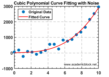
Example 5: Polynomial Curve Fitting with Noise
Fit a cubic polynomial to a set of noisy data points:
% Generate noisy data points

x = linspace(0, 10, 20);

y = 3*x.^3 - 2*x.^2 + x + 5 + randn(size(x))*100;


% Fit a cubic polynomial

p = polyfit(x, y, 3); % Third-degree polynomial

disp(p);


% Evaluate the fitted polynomial

x_fit = linspace(0, 10, 100);

y_fit = polyval(p, x_fit);


% Plot original data and fitted curve

plot(x, y, 'o', x_fit, y_fit, '-r');

legend('Original Data', 'Fitted Curve');

title('Cubic Polynomial Curve Fitting with Noise');
Explanation: This example demonstrates fitting a noisy dataset with a cubic polynomial and plotting the results for visualization.
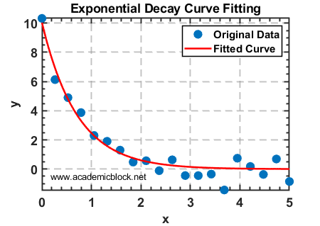
Example 6: Fitting an Exponential Decay
Model an exponential decay process using curve fitting:
% Generate synthetic data points

x = linspace(0, 5, 20);

y = 10 * exp(-1.5*x) + randn(size(x))*0.5;


% Fit an exponential decay curve

f = fit(x', y', 'exp1'); % Exponential model

disp(f);


% Plot original data and fitted curve

plot(x, y, 'o'); hold on;

plot(f, 'r-');

legend('Original Data', 'Fitted Curve');

title('Exponential Decay Curve Fitting');
Explanation: This example illustrates how to model an exponential decay process using MATLAB’s built-in fitting functions.
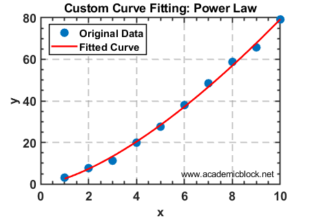
Example 7: Custom Curve Fitting for Power Law
Fit a power-law relationship y = a*x^b to a dataset:
% Data points

x = [1 2 3 4 5 6 7 8 9 10];

y = 2.5 * x.^1.5 + randn(size(x))*2;


% Define the custom model

ft = fittype('a*x^b', 'independent', 'x', 'coefficients', {'a', 'b'});

f = fit(x', y', ft);

disp(f);


% Plot original data and fitted curve

plot(x, y, 'o'); hold on;

plot(f, 'r-');

legend('Original Data', 'Fitted Curve');

title('Custom Curve Fitting: Power Law');
Explanation: This problem involves fitting a custom power-law model to the data using the fittype function.
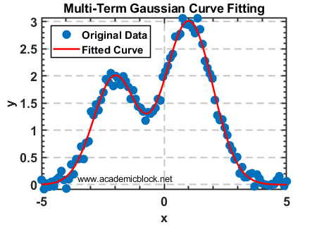
Example 8: Multi-Term Gaussian Fit
Fit a multi-term Gaussian model to simulated data:
% Generate data points

x = linspace(-5, 5, 100);

y = 3*exp(-(x-1).^2/2) + 2*exp(-(x+2).^2/1.5) + randn(size(x))*0.1;


% Fit a Gaussian model

ft = fittype('a1*exp(-((x-b1)^2)/(2*c1^2)) + a2*exp(-((x-b2)^2)/(2*c2^2))', ...

    'independent', 'x', 'coefficients', {'a1', 'b1', 'c1', 'a2', 'b2', 'c2'});

f = fit(x', y', ft, 'StartPoint', [3, 1, 1, 2, -2, 1]);

disp(f);


% Plot original data and fitted curve

plot(x, y, 'o'); hold on;

plot(f, 'r-');

legend('Original Data', 'Fitted Curve');

title('Multi-Term Gaussian Curve Fitting');
Explanation: This example shows how to fit a multi-term Gaussian model to complex data by defining a custom fitting equation.
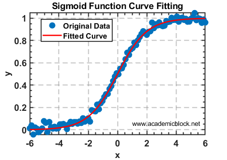
Example 9: Fitting a Sigmoid Function
Fit a logistic (sigmoid) function to a dataset:
% Generate data points

x = linspace(-6, 6, 100);

y = 1 ./ (1 + exp(-x)) + randn(size(x))*0.02;


% Define the custom sigmoid model

ft = fittype('1 / (1 + exp(-a*x + b))', ...

    'independent', 'x', 'coefficients', {'a', 'b'});

f = fit(x', y', ft, 'StartPoint', [1, 0]);

disp(f);


% Plot original data and fitted curve

plot(x, y, 'o'); hold on;

plot(f, 'r-');

legend('Original Data', 'Fitted Curve');

title('Sigmoid Function Curve Fitting');
Explanation: This example demonstrates fitting a logistic sigmoid function to data, often used in machine learning and biology.
Useful MATLAB Functions for Curve Fitting
polyfit(x, y, n) fits a polynomial of degree n to the data x and y.polyval(p, x) evaluates the polynomial p at the points in x.fit(x, y, model) fits a curve using the specified model (e.g., ‘poly1’, ‘exp1’).fittype(expression) creates a custom fitting type.lsqcurvefit performs non-linear curve fitting using least squares.Practice Questions
Test Yourself
1. Fit a cubic polynomial to the data x = [1 2 3 4 5] and y = [3 8 15 24 35].
2. Fit an exponential curve to the data x = [1 2 3 4 5] and y = [2 6 18 54 162].
3. Create and fit a custom model y = a*x2 + b*x + c to the data x = [1 2 3] and y = [2 6 12].
4. Fit a polynomial of degree 4 to a dataset with random noise added to y = x^4 - 3*x^3 + 2*x + 5.
5. Generate synthetic data for two overlapping Gaussian distributions and fit a two-term Gaussian model.
6. Fit an exponential growth model to the data x = [0 1 2 3 4 5] and y = [1 3 9 27 81 243].